Results
What each solver in Mosaic can do on each benchmark setup: whether its forward solution, gradient and optimization results are good enough for the task, what it costs relative to its peers, and how much of the campaign ran cleanly. Mosaic does not rank solvers or combine these into a single score.
These are example results, produced automatically on GitHub Actions runners and refreshed on every release. Accuracy and gradient metrics are hardware-independent and reproducible; wall-clock numbers reflect commodity cloud hardware and are best read as relative scaling between solvers. For numbers that reflect your setup, run the benchmarks yourself on your target hardware.
Each solver is wrapped in a Tesseract by the Mosaic team or its contributors. A flag or a slow time here says how this implementation behaves on this setup, not how good the underlying software is. The Effort column shows how far each wrapper had to go beyond documented use, and Deviations where it runs a substitute for part of the setup. Solvers that pass the same checks can differ a lot in how much work a new setup takes, so try the alternatives before committing to one.
If you maintain or use one of these solvers and can improve its configuration, contributions are welcome.
How to read the checks
Results are grouped by setup: one concrete problem statement, such as periodic Taylor–Green flow or channel flow past a cylinder. Setups of the same physics are not averaged, because a solver that handles one need not handle the other.
For each setup, each solver gets:
- Forward, gradient and optimization checks. Every experiment carries pass criteria set in its problem configuration (
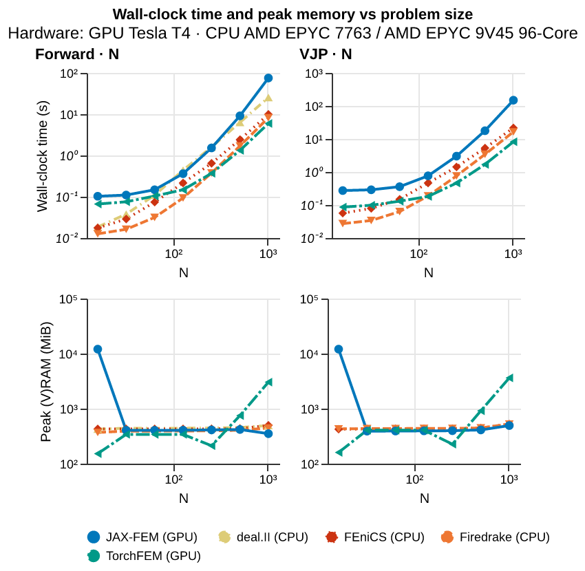
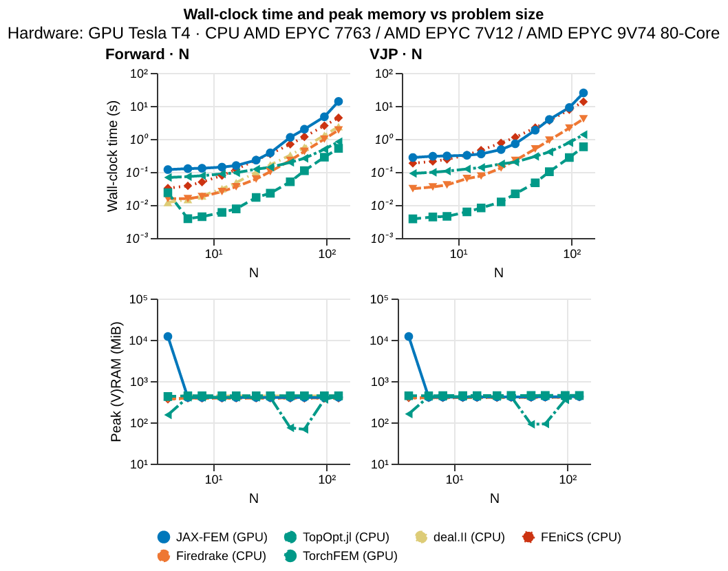
status_check): for example an error bound against the reference, a finite-difference agreement bound for the gradient, or the fraction of the objective an optimizer must remove. A check combines the setup’s gate experiments for that suite (see the table of states below). Hover a check for each gate’s headline numbers and the reasons for any flag; the list under each table spells the reasons out. - Cost, forward and VJP: wall-clock time as a multiple of the fastest solver on the same kind of device, at the largest problem size every solver in that group completed. GPU and CPU solvers ran on different machines, so they are compared within their group only; a solver sits in the group its cost results were measured on, and a note marks results that ran on another device than the solver now targets. A ≈ marks a gap to the fastest solver that is no larger than twice the spread (standard deviation) of the two solvers’ timed trials, so the two cannot be told apart on this run. Hover a cost for the mean, its spread, the number of trials and the first call, which includes compilation and setup. The per-suite tables on each results page give the absolute times.
- Reliability: how many of the setup’s experiments ran cleanly, out of those the solver supports, with flagged, failed, blocked and not-run experiments counted separately. This includes diagnostic experiments that are not gates (Jacobian spectra, horizon sweeps, cost sweeps). A cost run flagged only for being slow counts as clean here; its speed shows in the cost columns. Resource limits counts the sweeps a solver completed only up to some size or rollout length before running out of memory or time; where those limits lie depends on the hardware.
- Effort: the highest level among the interventions a solver needs on that setup, from L0 (documented options) and L1 (undocumented configuration) to L2 (user code on the library’s public primitives) and L3 (changes to the solver itself). A filter above the tables hides solvers above the level you are willing to work at yourself.
- Deviations: where a solver runs a substitute for the prescribed setup, such as a different outflow condition, with its effect on the results.
The Solver Reference lists every intervention with its reason, evidence and upstream issue, including those nobody has a reason for yet.
| State | Meaning |
|---|---|
| ✓ Pass | Every gate experiment met its criteria. |
| ! Borderline | A gate was flagged: it ran, but missed its criteria. A superscript i means every flag has a documented cause, often a property of the method or of the comparison rather than of the implementation; hover for the explanation. |
| ✗ Fail | A gate errored or produced no valid result. |
| ⊘ Blocked | The gates are excluded for a recorded reason that may be lifted: the solver is unstable on them, they are infeasible within the time or memory budget, an upstream bug stops them, or the wrapper does not implement them yet. The cell names the reason. |
| — Not supported | The method cannot express the experiment, e.g. a forward-only solver has no gradient. |
| · Not run | Not run in this campaign yet. |
Within each device group, solvers that pass more checks are listed first, then faster ones. That ordering is a reading aid, not a ranking: a solver that passes everything is not “better” than one that is flagged on a check your application does not need.
| Setup | Forward | Gradient | Optimization |
|---|---|---|---|
| H · Steady conduction in a slab | agreement, baseline, physical_laws, source_baseline, source_linearity |
fd_check, param_sweep, source_fd_check, source_width_sweep |
conductivity_recovery_bfgs |
| S · Linear-elastic cantilever | agreement, baseline, physical_laws |
fd_check, param_sweep |
topopt |
| F2 · Periodic box (Taylor–Green, multimode) | agreement, baseline, physical_laws, tgv_nu_sweep |
fd_check, analytic_check, analytic_check_nu, param_sweep |
— |
| F2 · Channel flow past a cylinder | cylinder |
— | drag_opt |
| F2 · Forced Kolmogorov flow | kolmogorov_laminar, kolmogorov |
chain_fd_check |
— |
| F3 · Triply periodic box (Taylor–Green) | agreement, baseline, physical_laws |
fd_check |
recovery |
Some criteria are absolute: an error bound against an analytic solution or a converged reference run, an observed order of convergence, or a minimum agreement with finite differences. Others compare a solver with the other solvers on the same experiment, for example an error more than three times the median of its peers. A flag on a relative criterion says that a solver is an outlier among its peers, not that it misses an accuracy the task needs. The thresholds are provisional and will be refined with the solver maintainers; they live next to each experiment in mosaic/benchmarks/problems/<domain>/config.py.
Checks by setup
Steady conduction in a slab
Heat transfer| Solver | Forward | Gradient | Optimization | Forward cost | VJP cost | Reliability | Effort | Deviations |
|---|---|---|---|---|---|---|---|---|
| GPU solvers · cost relative to the fastest GPU solver at N=1024, measured on Tesla T4 | ||||||||
| torch-fem | Pass | Pass | Pass | 1× (fastest) | 1× (fastest) | 14/14 ok | L0 | — |
| JAX-FEM | Pass | Pass | Pass | 13× | 18× | 14/14 ok | none | — |
| CPU solvers · cost relative to the fastest CPU solver at N=1024 | ||||||||
| Firedrake | Pass | Pass | Pass | 1× (fastest) | 1× (fastest) | 14/14 ok | none | — |
| FEniCS | Pass | Pass | Pass | 1.2× | 1.3× | 14/14 ok | L3 | — |
| deal.II | Pass | Not supported | Not supported | 3.1× | — | 7/7 ok | none | — |
Passes every check: Firedrake, torch-fem, FEniCS, JAX-FEM.
Not supported (1 solver)
- deal.II · 7 experiments — deal.II thermal tesseract is forward-only: this tesseract exposes no AD path (no VJP endpoint, no differentiable inputs), so cost/vjp and gradient experiments are categorically out of scope.; deal.II thermal tesseract exposes no AD path; conductivity recovery (gradient-based ρ updates that minimize the misfit to a target temperature field) requires a differentiable identification-error output.
Linear-elastic cantilever
Structural mechanics| Solver | Forward | Gradient | Optimization | Forward cost | VJP cost | Reliability | Effort | Deviations |
|---|---|---|---|---|---|---|---|---|
| GPU solvers · cost relative to the fastest GPU solver at N=128, measured on Tesla T4 | ||||||||
| torch-fem | Pass | Pass | Pass | 1× (fastest) | 1× (fastest) | 10/10 ok | L0 | — |
| FEniCSGPU run | Pass | Pass | Pass | 5.3× | 9.9× | 10/10 ok | none | — |
| JAX-FEM | Pass | Pass | Pass | 17× | 18× | 10/10 ok | none | — |
| CPU solvers · cost relative to the fastest CPU solver at N=128 | ||||||||
| TopOpt.jl | Pass | Pass | Pass | 1× (fastest) | 1× (fastest) | 10/10 ok | none | 1 |
| Firedrake | Pass | Pass | Pass | 3.6× | 7.0× | 10/10 ok | none | — |
| deal.II | Pass | Not supported | Not supported | 4.5× | — | 5/5 ok | none | — |
Passes every check: TopOpt.jl, torch-fem, Firedrake, FEniCS, JAX-FEM.
Not supported (1 solver)
- deal.II · 5 experiments — deal.II structural tesseract is forward-only: this tesseract exposes no AD path (no VJP endpoint, no differentiable inputs), so cost/vjp and gradient experiments are categorically out of scope.; deal.II structural tesseract has no AD path; topology-optimisation (compliance gradient-based ρ updates) requires a differentiable compliance output.
Periodic box (Taylor–Green, multimode)
Navier–Stokes (2D)| Solver | Forward | Gradient | Forward cost | VJP cost | Reliability | Effort | Deviations |
|---|---|---|---|---|---|---|---|
| GPU solvers · cost relative to the fastest GPU solver at N=256, measured on Tesla T4 | |||||||
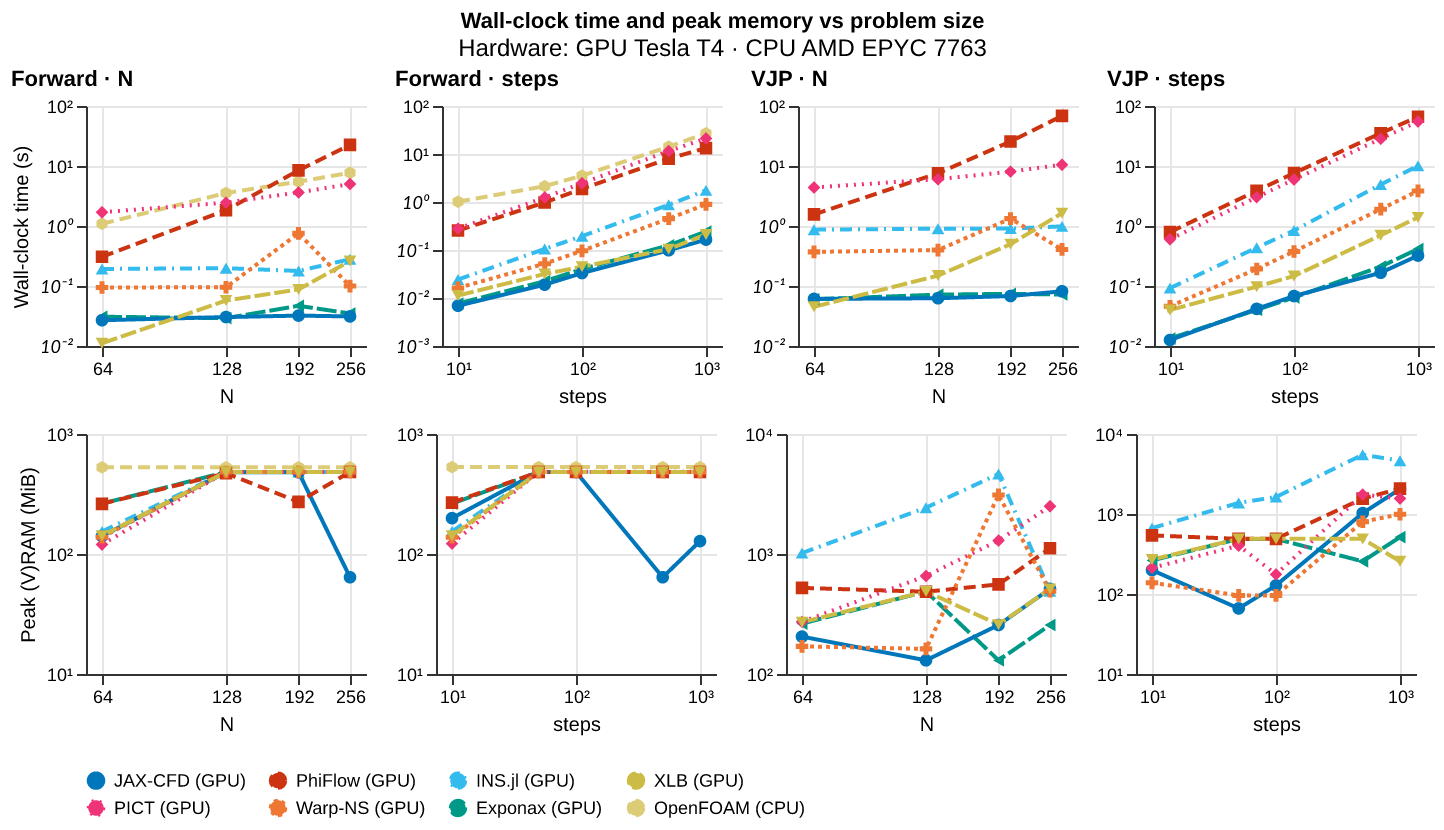
| jax-cfd | Pass | Pass | 1× (fastest) | ≈ 1.1× | 19/19 ok | none | — |
| Warp-NS | Pass | Pass | 3.2× | 5.6× | 19/19 ok | L2 | — |
| XLB | Pass | Pass | 8.4× | 23× | 19/19 ok | L2 | 1 |
| INS.jl | Pass | Pass | ≈ 9.0× | 14× | 19/19 ok | none | — |
| PhiFlow | Pass | Pass | 722× | 947× | 19/19 ok | L3 | — |
| Exponax | Borderlinei | Pass | 1.1× | 1× (fastest) | 18/19 ok1 flagged | L2 | — |
| PICT | Borderlinei | Pass | 161× | 146× | 18/19 ok1 flagged | L0 | — |
| CPU solvers · cost relative to the fastest CPU solver at N=256 | |||||||
| OpenFOAM | Borderline | Not supported | 1× (fastest) | — | 8/9 ok1 flagged | L0 | — |
Passes every check: jax-cfd, Warp-NS, XLB, INS.jl, PhiFlow.
Flags and exclusions (3)
- Exponax ·
forward/baseline· flagged — error converges at order -1.46 in N, below min_order=0.8 (explained: the Taylor–Green vortex is a single Fourier mode, which a spectral method represents exactly on every grid, so Exponax's error is float32 round-off from the first step. Round-off grows with the number of grid points and steps rather than shrinking with the grid spacing, so no positive order can be observed) - PICT ·
forward/baseline· flagged — error converges at order 0.35 in N, below min_order=0.8 (explained: PICT runs PISO with its default two pressure correctors, and its momentum predictor carries no pressure gradient. The splitting error this leaves scales with ν·dt/dx², which grows as the grid is refined at fixed CFL, so the error levels off on the finest grids and the observed order drops. More correctors remove the floor at a multiple of the wall time and reverse-mode memory) - OpenFOAM ·
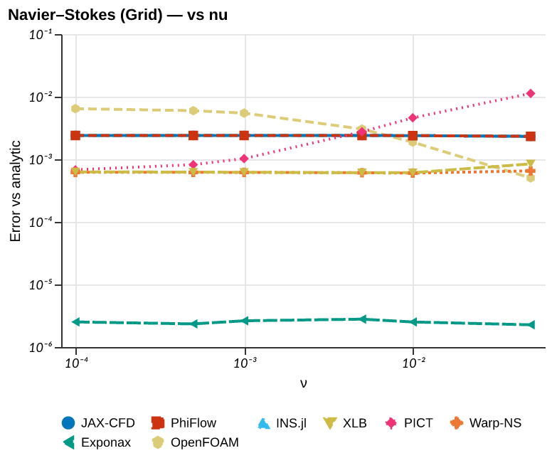
forward/tgv_nu_sweep· flagged — error 0.00645 at sweep=0.0001 is 4.2× peer median (0.00154); threshold k=3.0
Not supported (1 solver)
- OpenFOAM · 10 experiments — OpenFOAM has no VJP to benchmark; OpenFOAM is non-differentiable (C++, no AD path); DAFoam/OpenFOAM-AD exist but are not deployed in this tesseract
Channel flow past a cylinder
Navier–Stokes (2D)| Solver | Forward | Optimization | Reliability | Effort | Deviations |
|---|---|---|---|---|---|
| GPU solvers | |||||
| INS.jl | Pass | Pass | 2/2 ok | L2 | — |
| PhiFlow | Pass | Pass | 2/2 ok | L2 | — |
| Warp-NS | Pass | Pass | 2/2 ok | L2 | — |
| XLB | Pass | Pass | 2/2 ok | none | 1 |
| PICT | Pass | Infeasible | 1/2 ok1 infeasible | L2 | 1 |
| Exponax | Not supported | Not supported | — | none | — |
| jax-cfd | Not implemented | Not implemented | 0/2 ok2 not implemented | none | — |
| CPU solvers | |||||
| OpenFOAM | Pass | Not supported | 1/1 ok | L0 | — |
Passes every check: INS.jl, PhiFlow, Warp-NS, XLB.
Flags and exclusions (3)
- PICT ·
optimization/drag_opt· infeasible — each drag_opt iteration runs a full forward and VJP through PICT's unpreconditioned pressure solves on the body-fitted channel mesh, so the experiment takes hours on the benchmark GPU - jax-cfd ·
forward/cylinder· not implemented — jax-cfd 0.2.1 cannot express the channel through its API. Its advection raises NotImplementedError for any inflow (only no-penetration and periodic boundaries are supported), it pads a zero-gradient boundary only for cell-centered fields, so the outlet's face-centered u_x cannot have one, its boundary values are scalars, so the inlet cannot carry a profile, and it has no obstacles. Running it would take a hand-written convection, inlet and outlet conditions and obstacle on jax-cfd's grid primitives, which this tesseract does not have - jax-cfd ·
optimization/drag_opt· not implemented — jax-cfd 0.2.1 cannot express the channel through its API. Its advection raises NotImplementedError for any inflow (only no-penetration and periodic boundaries are supported), it pads a zero-gradient boundary only for cell-centered fields, so the outlet's face-centered u_x cannot have one, its boundary values are scalars, so the inlet cannot carry a profile, and it has no obstacles. Running it would take a hand-written convection, inlet and outlet conditions and obstacle on jax-cfd's grid primitives, which this tesseract does not have
Not supported (2 solvers)
- OpenFOAM · 1 experiments — OpenFOAM is a non-differentiable, forward-only solver
- Exponax · 2 experiments — a Fourier pseudo-spectral method represents only periodic fields, so it cannot express a channel with walls, an inflow and an outflow
Triply periodic box (Taylor–Green)
Navier–Stokes (3D)| Solver | Forward | Gradient | Optimization | Forward cost | VJP cost | Reliability | Effort | Deviations |
|---|---|---|---|---|---|---|---|---|
| GPU solvers · cost relative to the fastest GPU solver at N=64, measured on Tesla T4 | ||||||||
| INS.jl | Pass | Pass | Pass | 1× (fastest) | 1× (fastest) | 16/16 ok1 resource limit | none | — |
| XLB | Pass | Pass | Pass | 1.7× | ≈ 1.4× | 16/16 ok1 resource limit | L2 | 1 |
| Exponax | Pass1/5 | Pass | Pass | — | — | 8/16 ok8 not run | none | — |
| jax-cfd | Pass1/5 | Pass | Pass | — | — | 8/16 ok8 not run1 resource limit | none | — |
| PhiFlow | Pass1/5 | Pass | Pass | — | — | 8/16 ok8 not run1 resource limit | L3 | — |
| PICT | Pass1/5 | Pass | Pass | — | — | 8/16 ok8 not run1 resource limit | none | — |
| Warp-NS | Pass1/5 | Pass | Pass | — | — | 8/16 ok8 not run1 resource limit | L2 | — |
| CPU solvers · cost relative to the fastest CPU solver | ||||||||
| OpenFOAM | Pass1/5 | Not supported | Not supported | — | — | 1/7 ok6 not run | none | — |
Passes every check: INS.jl, XLB, Exponax, jax-cfd, PhiFlow, PICT, Warp-NS.
Flags and exclusions (46)
- Exponax ·
forward/agreement· not run - Exponax ·
forward/physical_laws/vs_N· not run - Exponax ·
forward/physical_laws/vs_nu· not run - Exponax ·
forward/physical_laws/vs_steps· not run - Exponax ·
cost/spatial_cost· not run - Exponax ·
cost/temporal_cost· not run - Exponax ·
cost/vjp_cost/by_N· not run - Exponax ·
cost/vjp_cost/by_steps· not run - jax-cfd ·
forward/agreement· not run - jax-cfd ·
forward/physical_laws/vs_N· not run - jax-cfd ·
forward/physical_laws/vs_nu· not run - jax-cfd ·
forward/physical_laws/vs_steps· not run - jax-cfd ·
cost/spatial_cost· not run - jax-cfd ·
cost/temporal_cost· not run - jax-cfd ·
cost/vjp_cost/by_N· not run - jax-cfd ·
cost/vjp_cost/by_steps· not run - PhiFlow ·
forward/agreement· not run - PhiFlow ·
forward/physical_laws/vs_N· not run - PhiFlow ·
forward/physical_laws/vs_nu· not run - PhiFlow ·
forward/physical_laws/vs_steps· not run - PhiFlow ·
cost/spatial_cost· not run - PhiFlow ·
cost/temporal_cost· not run - PhiFlow ·
cost/vjp_cost/by_N· not run - PhiFlow ·
cost/vjp_cost/by_steps· not run - PICT ·
forward/agreement· not run - PICT ·
forward/physical_laws/vs_N· not run - PICT ·
forward/physical_laws/vs_nu· not run - PICT ·
forward/physical_laws/vs_steps· not run - PICT ·
cost/spatial_cost· not run - PICT ·
cost/temporal_cost· not run - PICT ·
cost/vjp_cost/by_N· not run - PICT ·
cost/vjp_cost/by_steps· not run - Warp-NS ·
forward/agreement· not run - Warp-NS ·
forward/physical_laws/vs_N· not run - Warp-NS ·
forward/physical_laws/vs_nu· not run - Warp-NS ·
forward/physical_laws/vs_steps· not run - Warp-NS ·
cost/spatial_cost· not run - Warp-NS ·
cost/temporal_cost· not run - Warp-NS ·
cost/vjp_cost/by_N· not run - Warp-NS ·
cost/vjp_cost/by_steps· not run - OpenFOAM ·
forward/agreement· not run - OpenFOAM ·
forward/physical_laws/vs_N· not run - OpenFOAM ·
forward/physical_laws/vs_nu· not run - OpenFOAM ·
forward/physical_laws/vs_steps· not run - OpenFOAM ·
cost/spatial_cost· not run - OpenFOAM ·
cost/temporal_cost· not run
Resource limits (6)
Sweeps a solver completed only up to some size or rollout length: it ran out of memory or time, or, in sweeps that look for the limit, failed past the last value it completed. Unless that happened at the first value, the experiment counts as ok; the limit shows how far the solver goes on this hardware.
- INS.jl ·
gradient/horizon_sweep_limits· from steps=5120 - XLB ·
gradient/horizon_sweep_limits· from steps=320 - jax-cfd ·
gradient/horizon_sweep_limits· from steps=5120 - PhiFlow ·
gradient/horizon_sweep_limits· from steps=160 - PICT ·
gradient/horizon_sweep_limits· from steps=10240 - Warp-NS ·
gradient/horizon_sweep_limits· from steps=160
Not supported (1 solver)
- OpenFOAM · 9 experiments — standard icoFoam has no VJP to benchmark; standard icoFoam is non-differentiable (C++, no AD path); DAFoam/OpenFOAM-AD exist but are not deployed in this tesseract; standard icoFoam is a non-differentiable, forward-only solver
Domains
Each domain page collects the setups of one physics problem and reports, per suite: forward (output against a trusted reference, and an analytic solution where one exists), gradient (AD or adjoint gradient against a finite-difference ground truth, in magnitude and direction), cost (forward and VJP wall-clock scaling with problem size) and optimization (end-to-end convergence using each solver’s own gradients). See the Overview for the full evaluation protocol.
F2
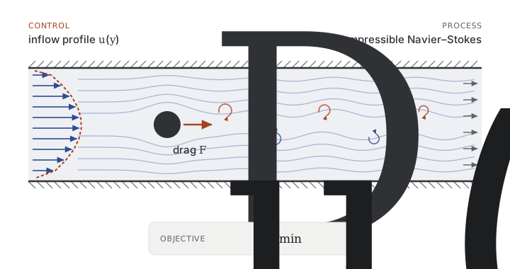
Optimize the inflow of a 2D channel flow to minimize drag on a cylinder, differentiating through an incompressible fluid solver. Covers JAX-CFD, PhiFlow, INS.jl, XLB, PICT, Warp-NS, and OpenFOAM across spectral, finite-difference, finite-volume, and LBM schemes.
F3
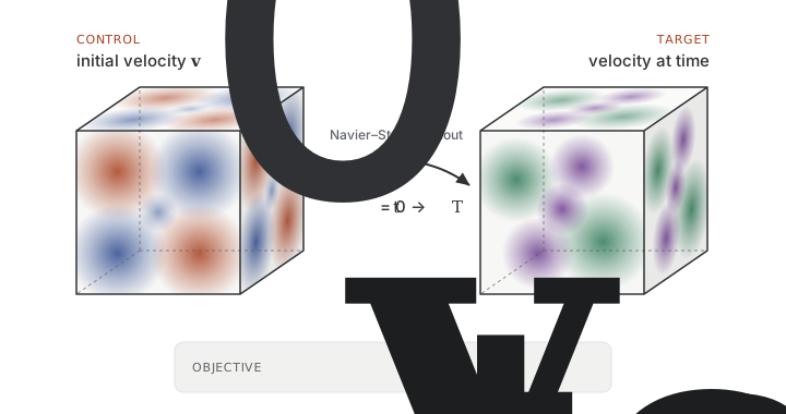
Recover the initial velocity field of a 3D turbulent flow from a later snapshot, differentiating through the Navier–Stokes rollout. Covers PhiFlow, XLB, PICT, Warp-NS, Exponax, INS.jl, and OpenFOAM on a triply periodic Taylor–Green vortex.
S
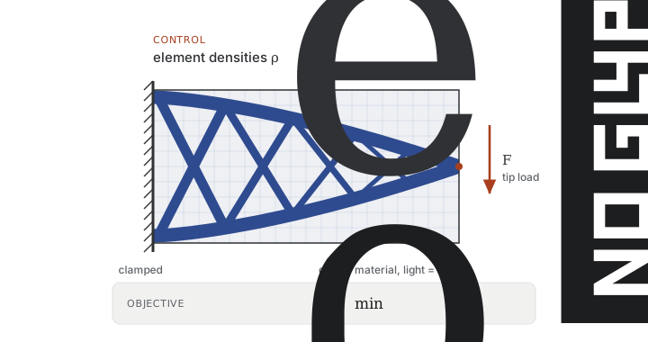
Place a fixed budget of material in a clamped beam to make it as stiff as possible, differentiating through a finite-element solve. Covers deal.II, FEniCS, Firedrake, JAX-FEM, TopOpt.jl, and torch-fem on 2D cantilever compliance minimization with SIMP penalization.
H
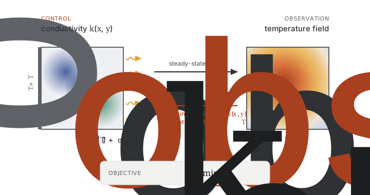
Invert for the conductivity field of a slab from its temperature, differentiating through a steady heat-conduction solve. Covers deal.II, FEniCS, Firedrake, JAX-FEM, and torch-fem on 2D steady-state heat conduction.
Experiment explorer
Every experiment across all domains. Search or filter, then click a card to see its plots.
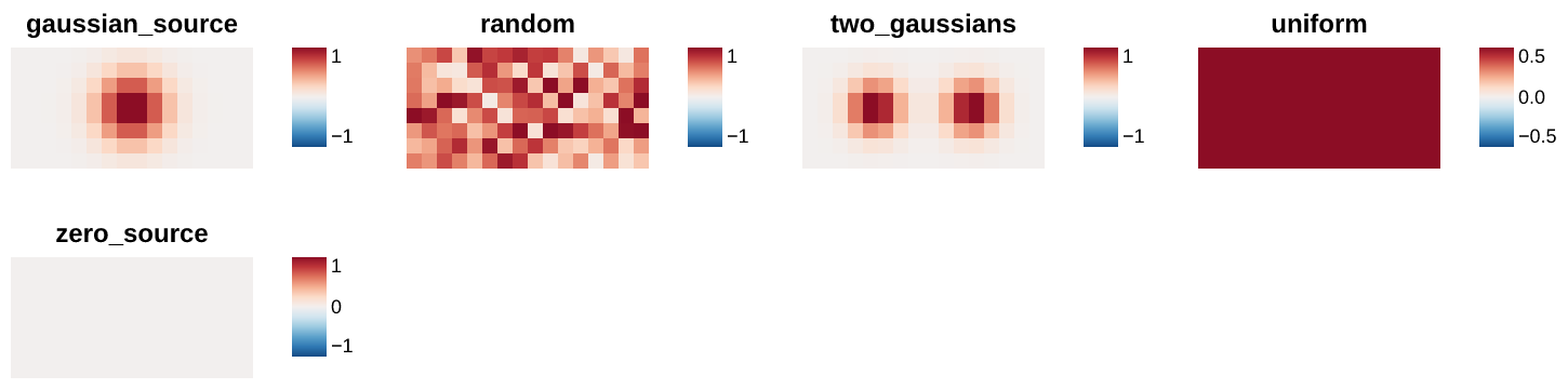
H Initial Conditions 1 plot
Initial Conditions overview
H Forward 1 plot
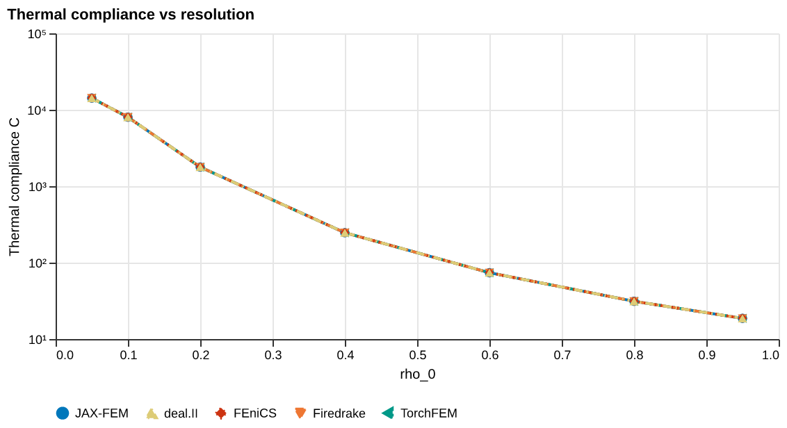
Agreement
Heat transfer · Forward
Thermal compliance \(C\) vs uniform element density \(\rho_0\) at fixed \(N\); compares solvers on a log scale.
H Forward 1 plot
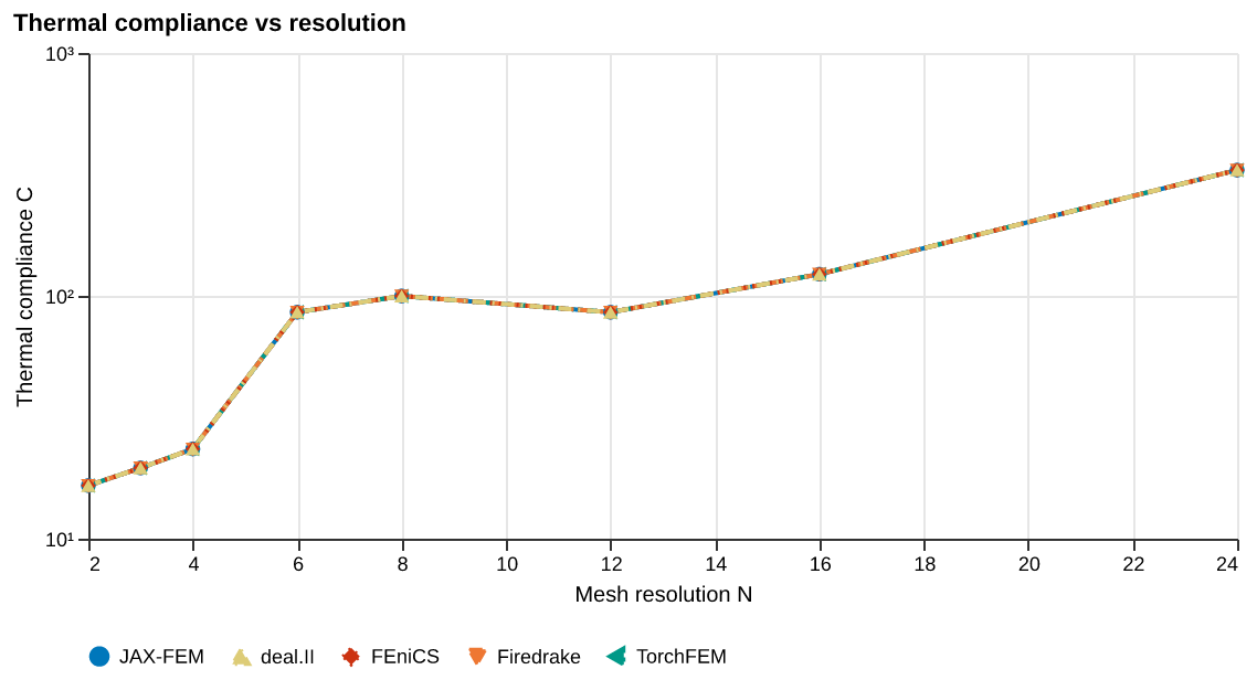
Baseline
Heat transfer · Forward
Thermal compliance \(C\) vs mesh resolution \(N\) with random density; compares FV and FEM solvers across refinements.
H Forward 1 plot
Physical Laws
Heat transfer · Forward
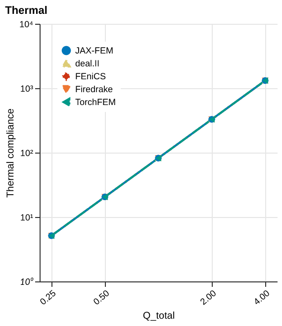
Thermal compliance \(C\) vs total heat flux \(Q_\mathrm{total}\) at fixed \(N\) and \(\rho_0\) with a hot-spot BC; shown on log-log axes.
H Forward 1 plot
Source Baseline
Heat transfer · Forward
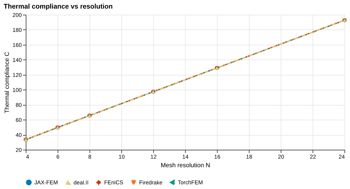
Thermal compliance \(C\) vs mesh resolution \(N\) with a Gaussian source field; compares solvers across refinements.
H Forward 1 plot
Source Linearity
Heat transfer · Forward
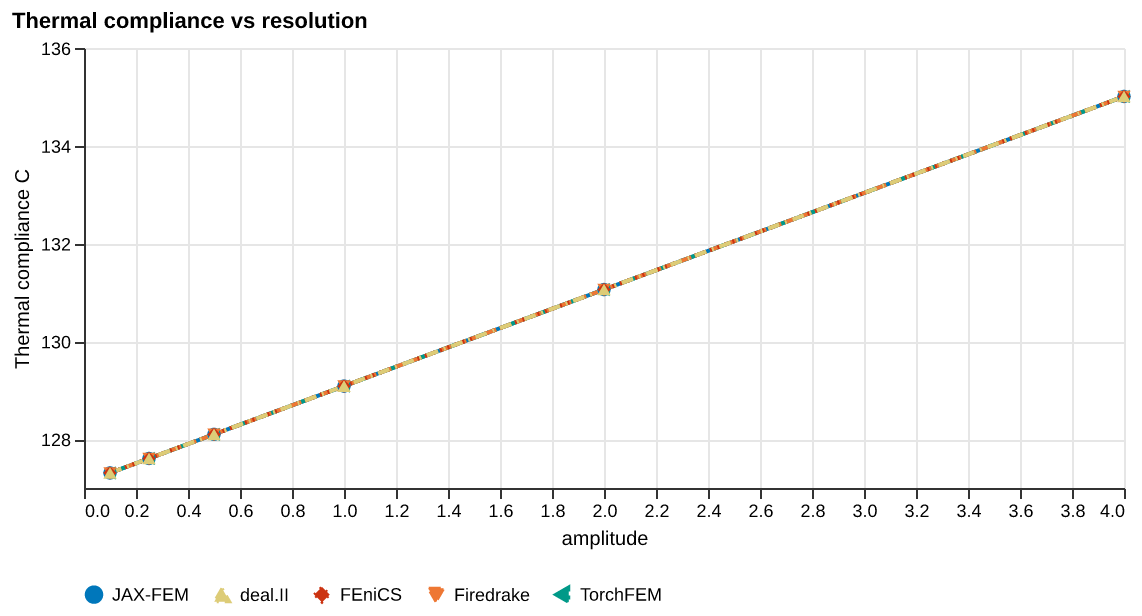
Thermal compliance \(C\) vs source amplitude at fixed mesh; compares solvers on log-log axes.
H Gradient 1 plot
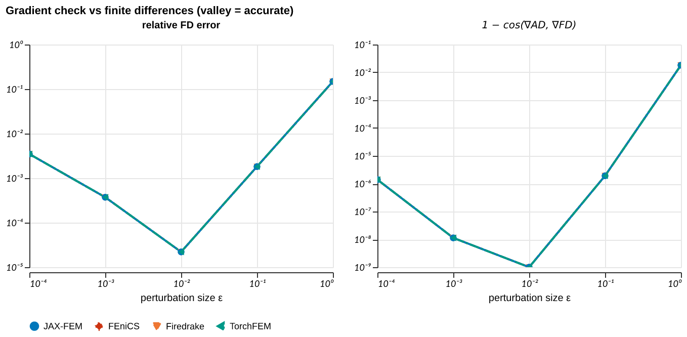
Finite-Difference Check
Heat transfer · Gradient
FD gradient error vs step size \(\varepsilon\) (U-curves), AD/FD direction cosine, and gradient magnitude field panels.
H Gradient 1 plot
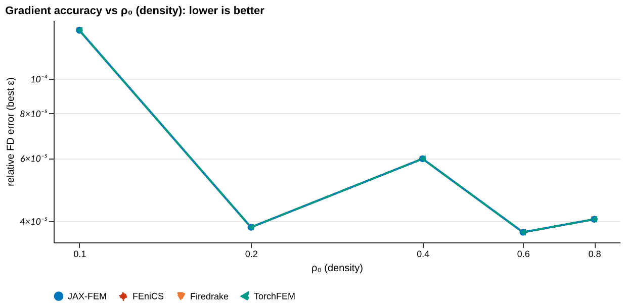
Parameter Sweep
Heat transfer · Gradient
Gradient norm, best-\(\varepsilon\) FD error, AD/FD direction cosine, and U-curves vs element density \(\rho_0\).
H Gradient 1 plot
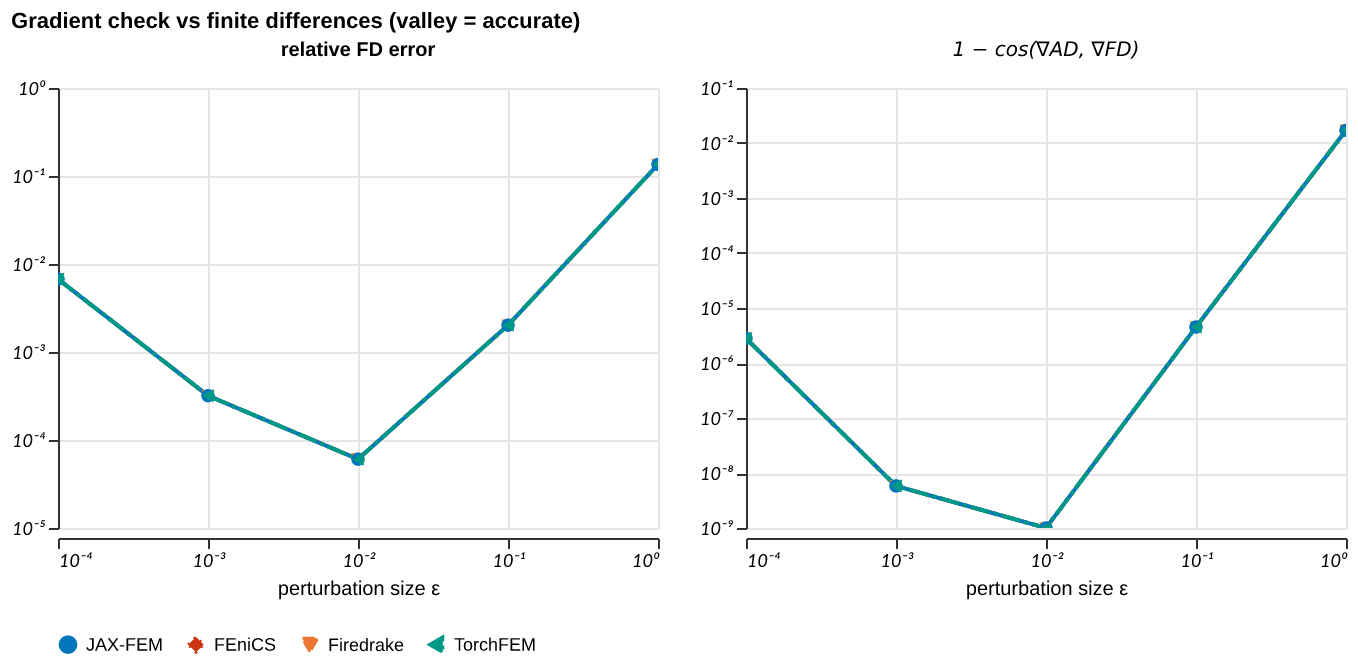
Source Fd Check
Heat transfer · Gradient
FD gradient error vs \(\varepsilon\), AD/FD direction cosine, and gradient field panels for d(identification_error)/d(source).
H Gradient 1 plot
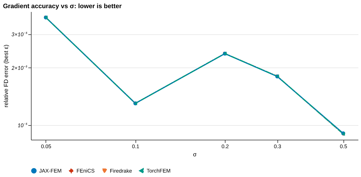
Source Width Sweep
Heat transfer · Gradient
Gradient norm, best-\(\varepsilon\) FD error, AD/FD direction cosine, and U-curves vs source width \(\sigma\).
H Optimization 1 plot
Conductivity Recovery (L-BFGS)
Heat transfer · Optimization
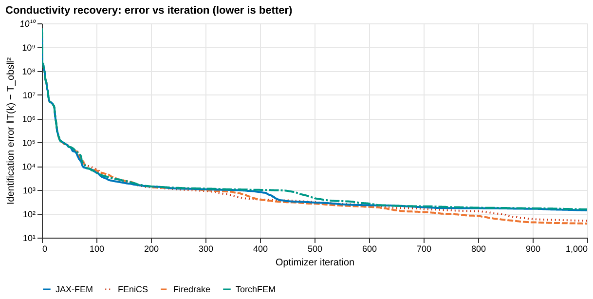
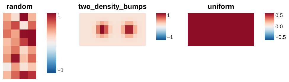
Optimisation traces (loss vs iteration) and recovered conductivity fields vs the two-Gaussian ground truth, using L-BFGS.
S Initial Conditions 1 plot
Initial Conditions overview
S Forward 1 plot
Agreement
Structural mechanics · Forward
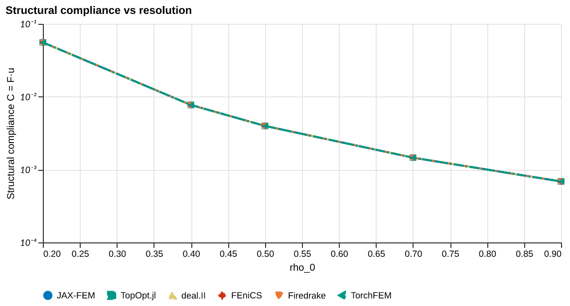
Structural compliance \(C = \mathbf{F}^\top \mathbf{u}\) vs density \(\rho_0\) at fixed mesh, sweeping uniform density to span the SIMP stiffness regime.
S Forward 1 plot
Baseline
Structural mechanics · Forward
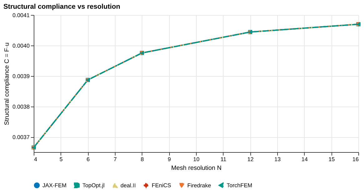
Structural compliance \(C = \mathbf{F}^\top \mathbf{u}\) vs mesh resolution \(N\) for each solver, uniform density \(\rho_0=0.5\), full-face downward load.
S Forward 1 plot
Physical Laws
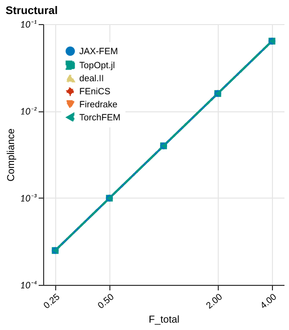
Structural mechanics · Forward
Diagnostic functionals (compliance, total displacement) vs total load \(F_\mathrm{total}\), validating linearity of the SIMP response.
S Gradient 1 plot
Finite-Difference Check
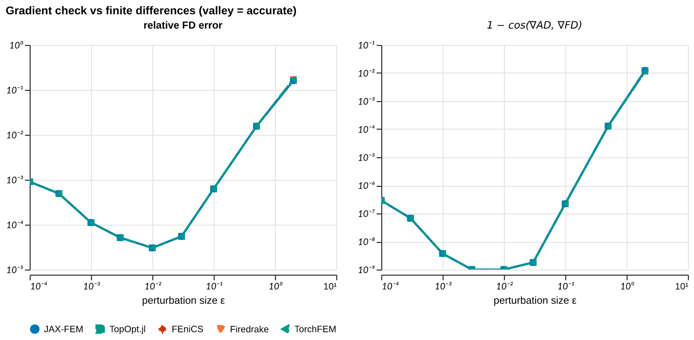
Structural mechanics · Gradient
U-curves of finite-difference gradient error vs perturbation size \(\varepsilon\) with subspace cosine, validating VJP correctness on a random density.
S Gradient 1 plot
Parameter Sweep
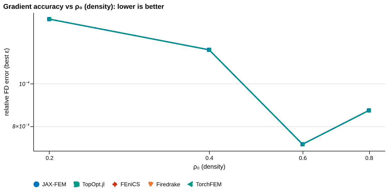
Structural mechanics · Gradient
Gradient norm, best-\(\varepsilon\) FD error, direction cosine, and U-curves vs uniform density \(\rho_0\).

S Optimization 8 plots
Topology Optimisation
Structural mechanics · Optimization
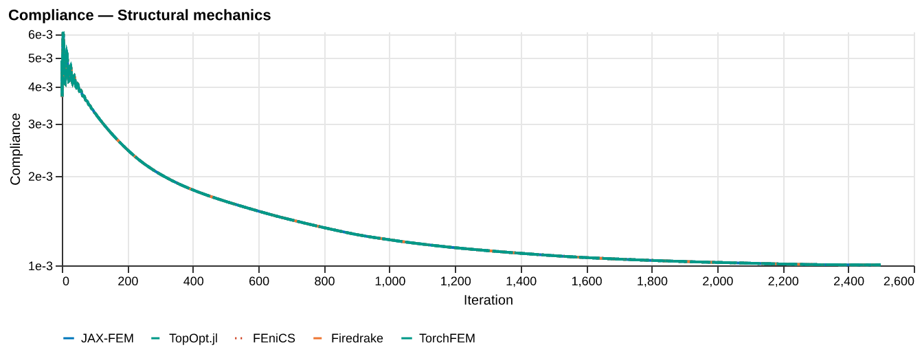
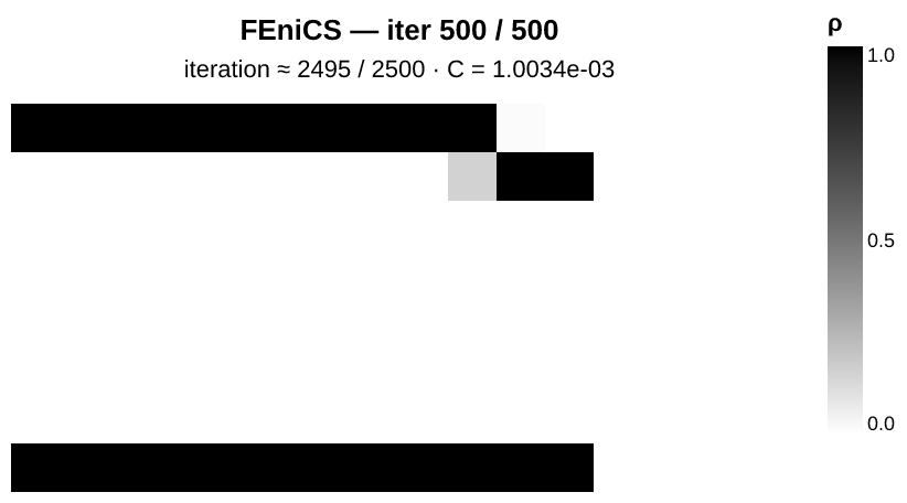
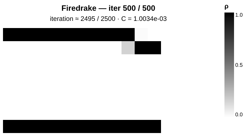
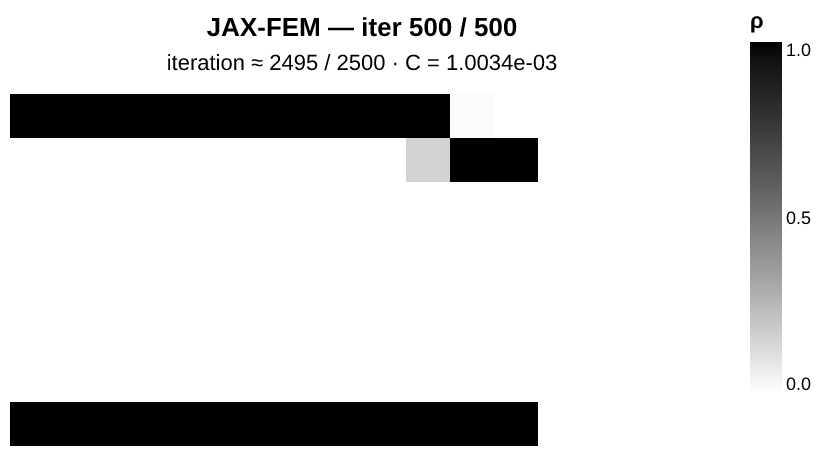
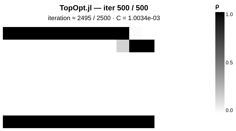
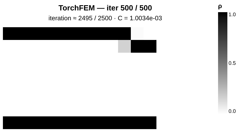
SIMP topology optimisation on a \(16\times8\times8\) cantilever beam with Adam (lr=0.05): compliance \(C = \mathbf{F}^\top \mathbf{u}\) and density field evolution under a 50% volume-fraction constraint.


F2 Initial Conditions 1 plot
Initial Conditions overview
F2 Forward 1 plot
Baseline
Navier–Stokes (2D) · Forward
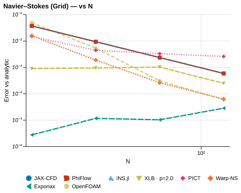
Relative error vs grid resolution \(N\) against the analytic TGV solution at \(t=1.28\), refining space and time together at a fixed CFL number. The legend gives each solver’s observed order of accuracy \(p\).
F2 Forward 1 plot
Cylinder
Navier–Stokes (2D) · Forward
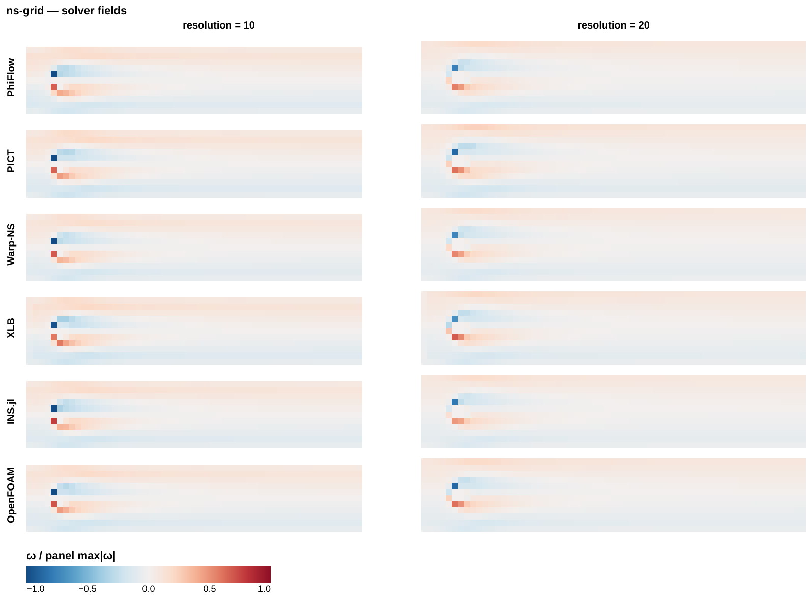
Steady flow past a cylinder in a channel (Schäfer–Turek DFG 2D-1, Re = 20) at 10 and 20 cells per diameter. Each solver’s drag coefficient at 20 is scored against the reference Cd = 5.5795. The pressure difference across the cylinder (reference 0.1175) and the lift coefficient are also reported. The vorticity fields are for visual comparison.
F2 Forward 1 plot
Tgv Nu Sweep
Navier–Stokes (2D) · Forward
Relative error vs viscosity \(\nu\) for each solver at a fixed TGV initial condition.
F2 Gradient 1 plot
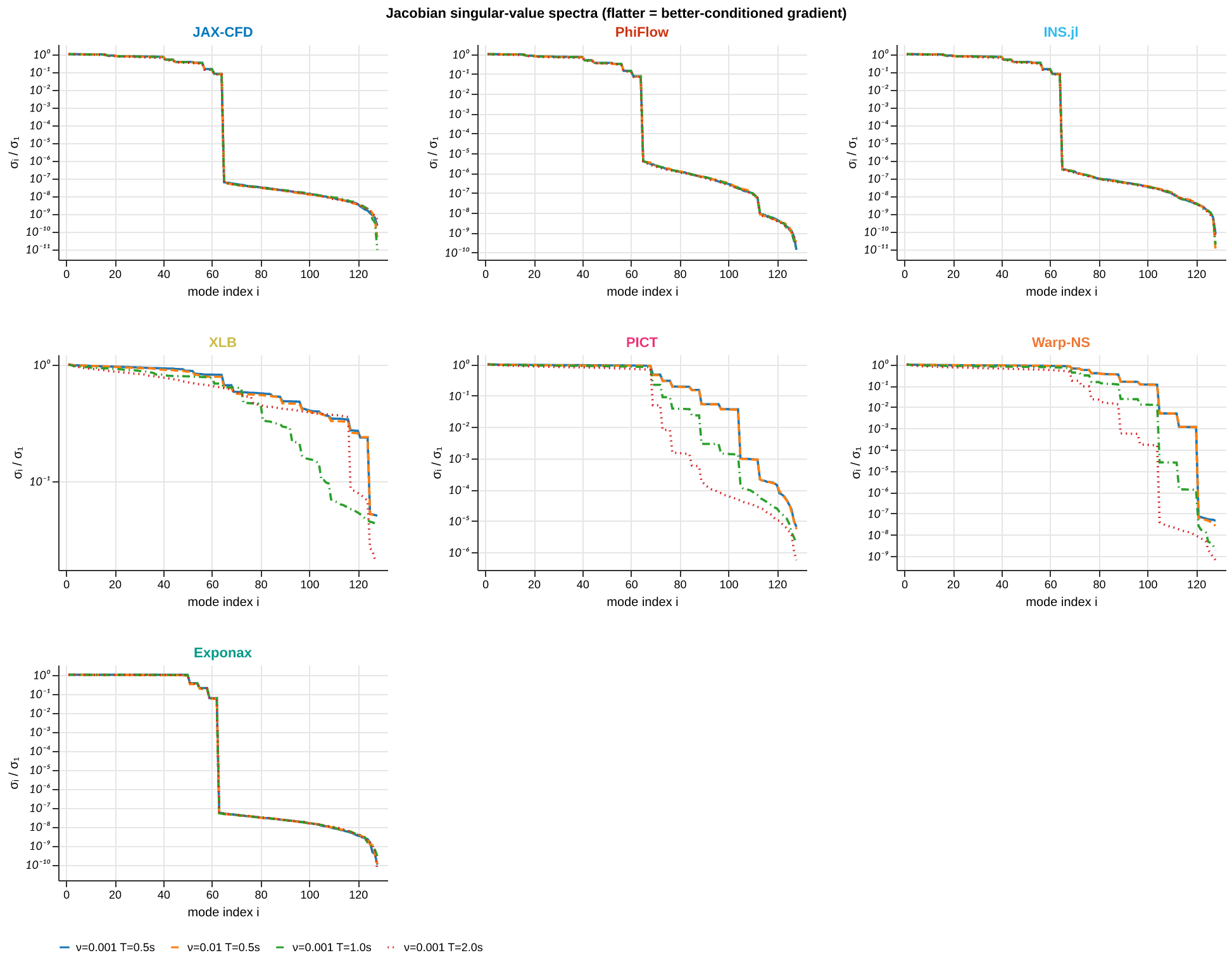
Gradient overview
F2 Gradient 2 plots
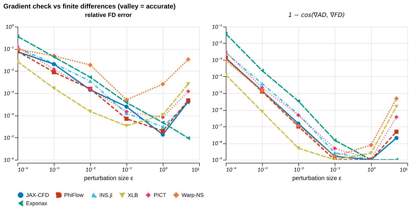
Finite-Difference Check
Navier–Stokes (2D) · Gradient
U-curves of finite-difference gradient error vs perturbation size \(\varepsilon\) together with subspace cosine; validates VJP correctness.
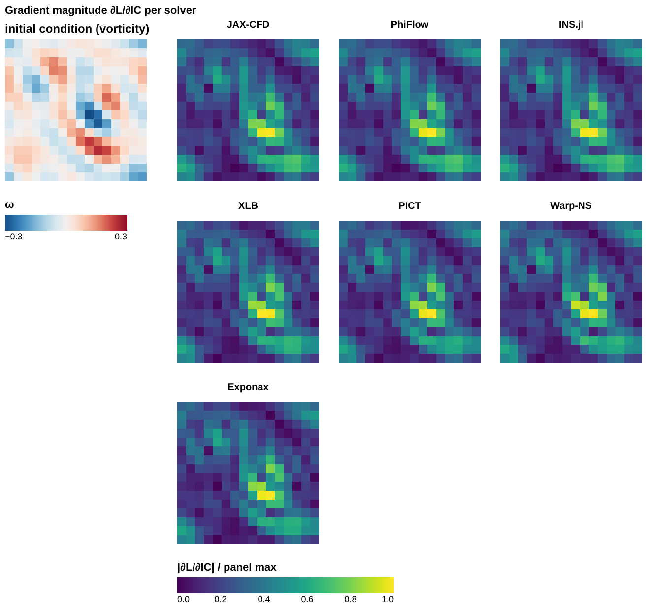
F2 Gradient 1 plot
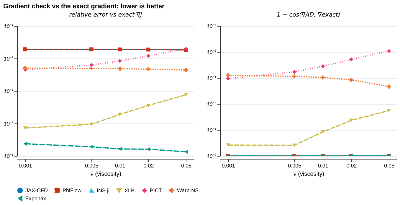
Analytic Gradient Check
Navier–Stokes (2D) · Gradient
Relative error and 1 − cosine of each solver’s gradient of \(J = \sum \lvert\mathbf{u}(T)\rvert^2\) with respect to the TGV initial field, against the exact gradient \(\nabla J = 2 e^{-4\nu T}\,\mathbf{u}_0\). The closed form holds for divergence-free perturbations, so each gradient is compared after projecting out its curl-free part. There is no finite-difference step to tune, but the error includes the forward discretization error.
F2 Gradient 1 plot
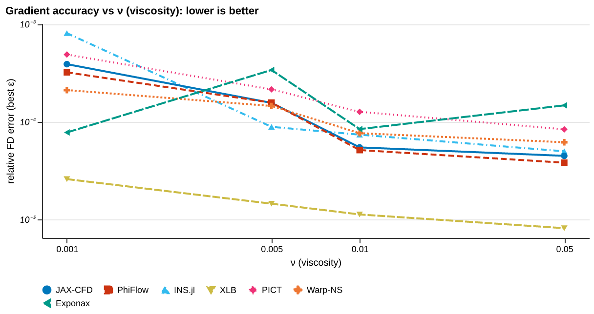
Parameter Sweep
Navier–Stokes (2D) · Gradient
Gradient norm, best-\(\varepsilon\) FD error, direction cosine, and U-curves vs the sweep parameter.
F2 Gradient 1 plot
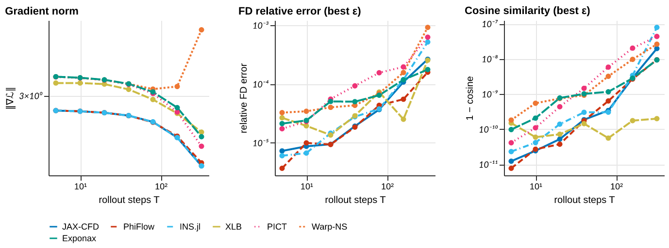
Horizon Sweep
Navier–Stokes (2D) · Gradient
Gradient norm, FD error, and direction cosine vs rollout horizon \(T = \mathrm{steps}\cdot dt\).
F2 Optimization 3 plots
Drag Optimisation
Navier–Stokes (2D) · Optimization
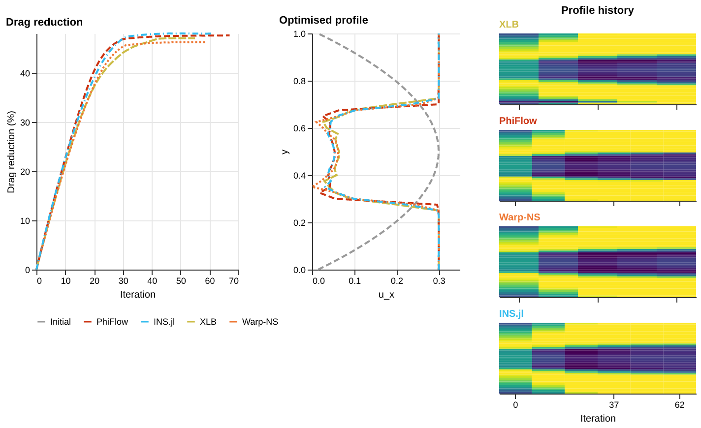
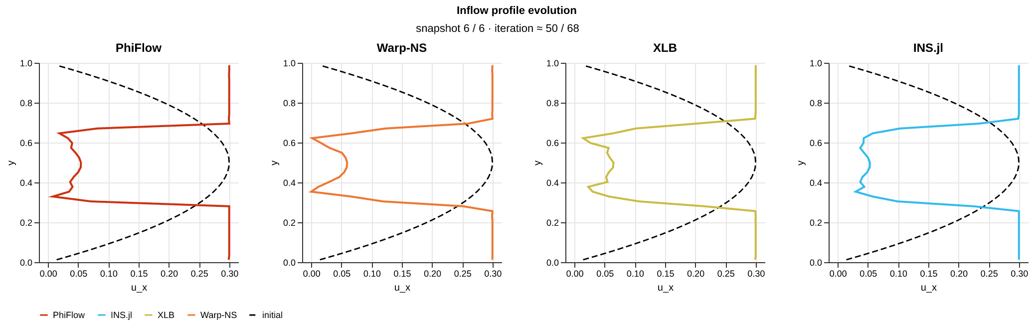
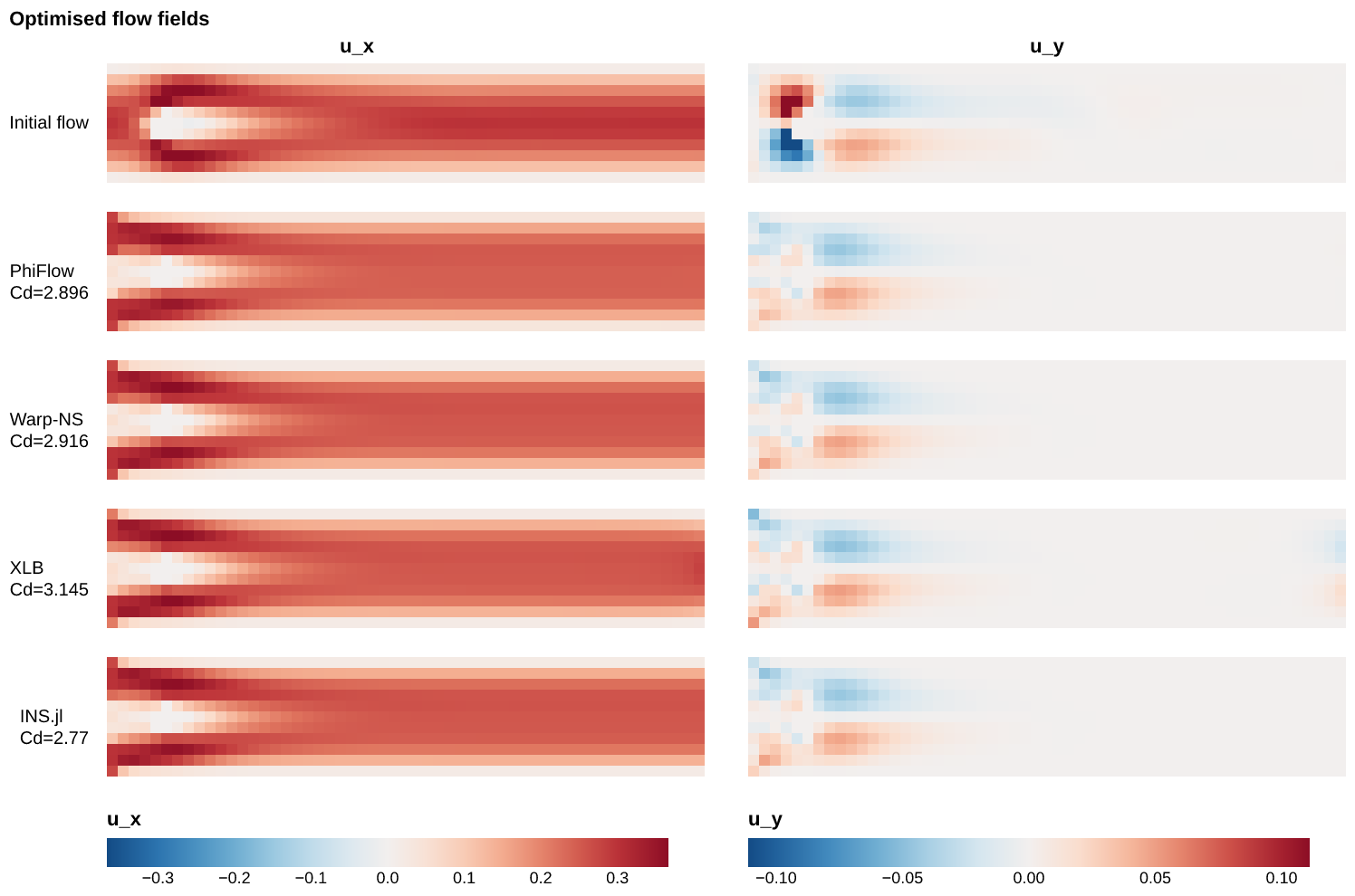
Drag minimization over the inlet profile of the DFG 2D-1 channel at a fixed flow rate: drag coefficient per iteration, optimized vs initial inflow profiles, and the flow fields before and after.
F3 Initial Conditions 1 plot
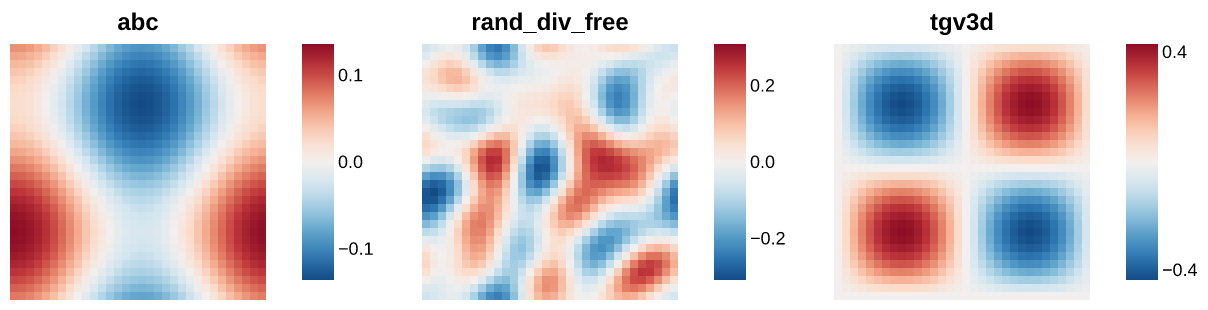
Initial Conditions overview
F3 Forward 1 plot
Agreement
Navier–Stokes (3D) · Forward
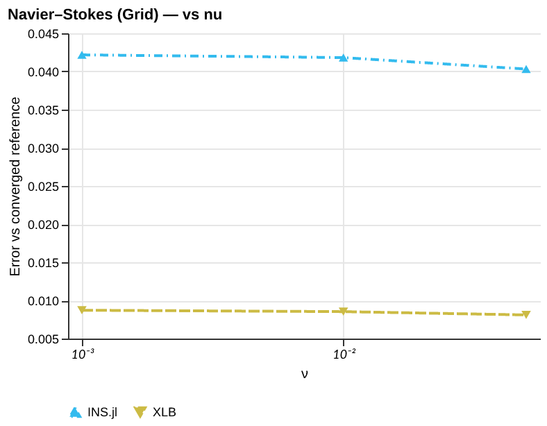
3D velocity magnitude fields and kinetic energy spectra per solver, swept over viscosity ν, compared against a converged spectral reference. (The 3D TGV initial condition is not advection-free, so the linearized analytic decay is only a short-horizon consistency check, not an accuracy reference.) The reference is an Exponax run at N=64, spectrally truncated to N=16. Exponax’s low error here, and its top place in the forward ranking, therefore largely measure agreement with its own higher-resolution solution.
F3 Forward 1 plot
Baseline
Navier–Stokes (3D) · Forward
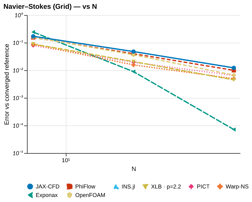
Relative error vs grid resolution N against a converged spectral reference at t=1.28, refining space and time together at a fixed CFL number. The legend gives each solver’s observed order of accuracy p.
F3 Gradient 1 plot
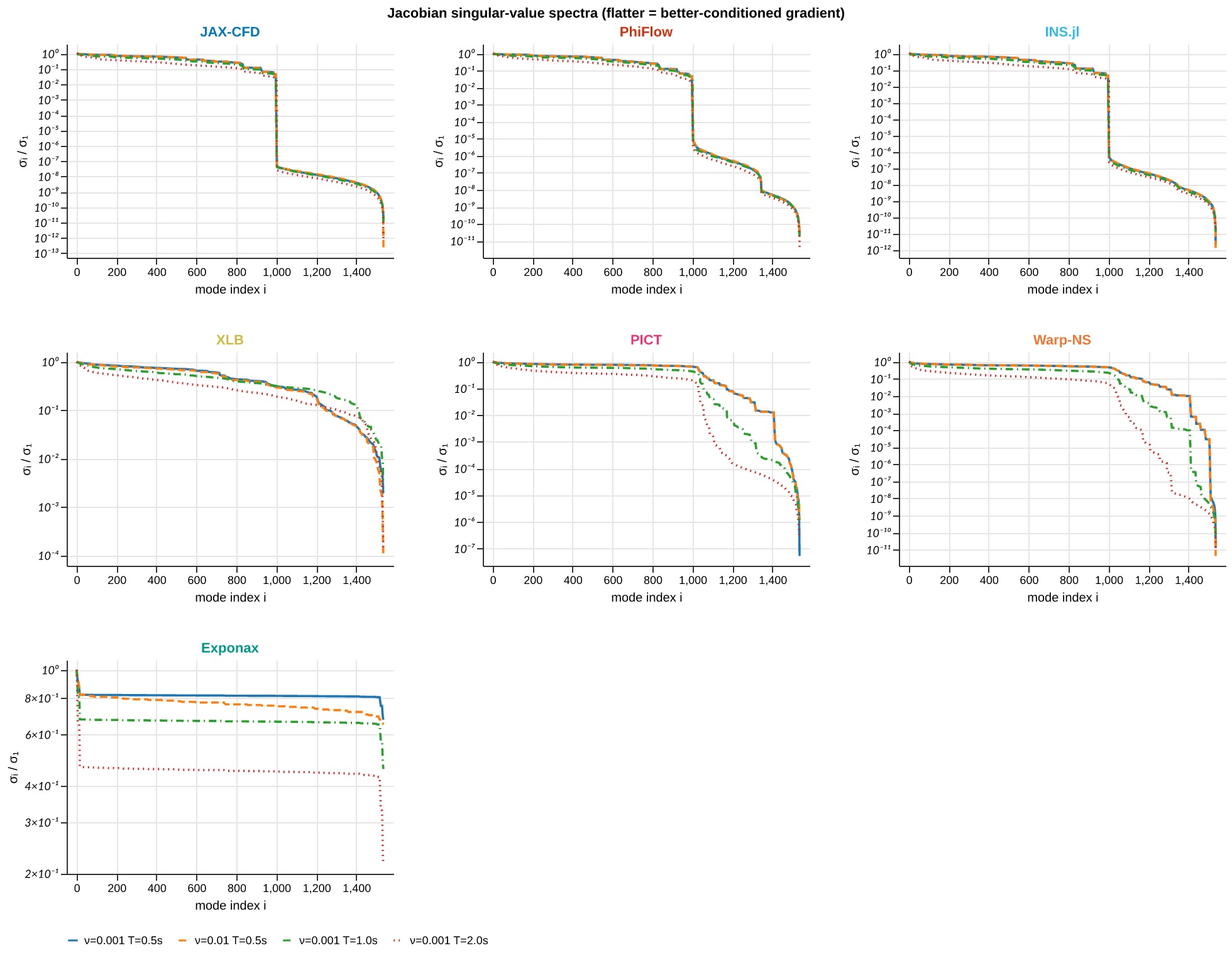
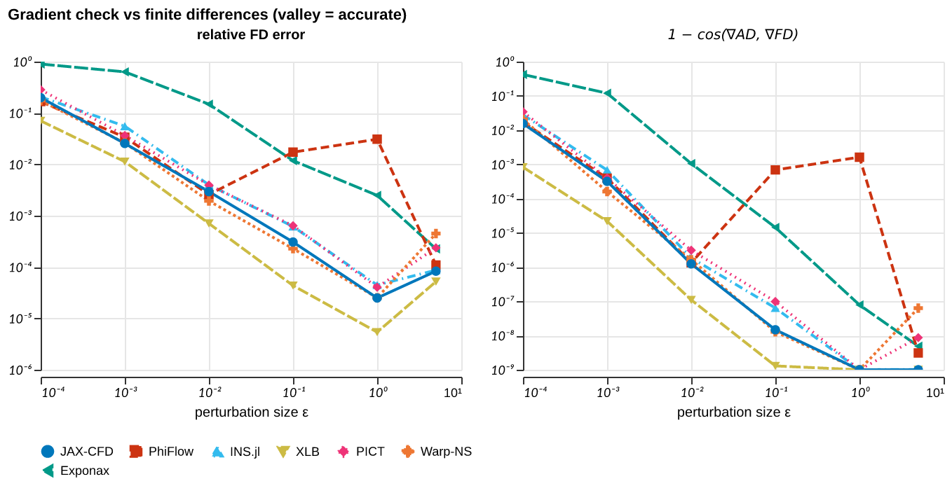
Gradient overview
F3 Gradient 2 plots
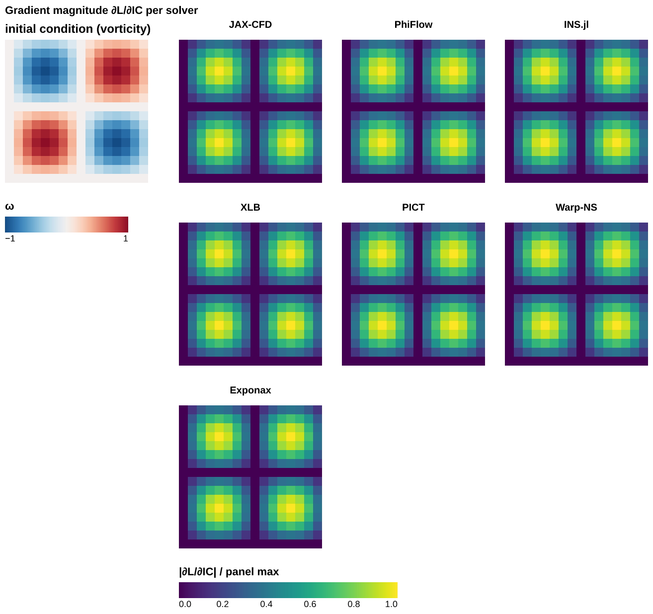
Finite-Difference Check
Navier–Stokes (3D) · Gradient
Finite-difference gradient error U-curves and direction cosine vs perturbation ε for each solver on the 3D Taylor-Green vortex IC.
F3 Gradient 1 plot
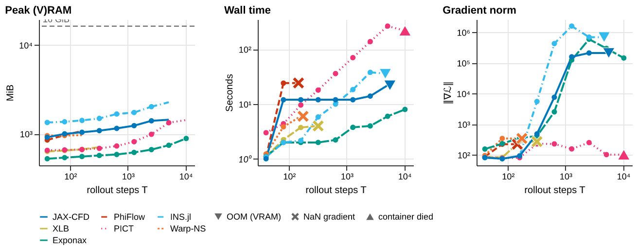
Horizon Sweep Limits
Navier–Stokes (3D) · Gradient
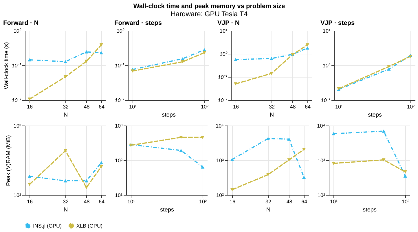
Per-solver rollout-limit table reporting step count at first failure, failure type, and wall time per successful step.
F3 Optimization 2 plots
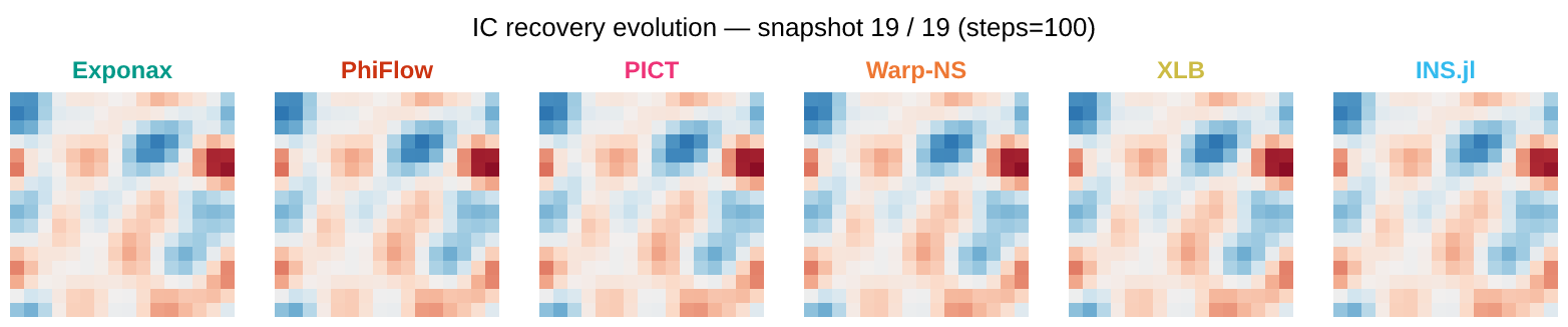
Initial-Condition Recovery (L-BFGS)
Navier–Stokes (3D) · Optimization
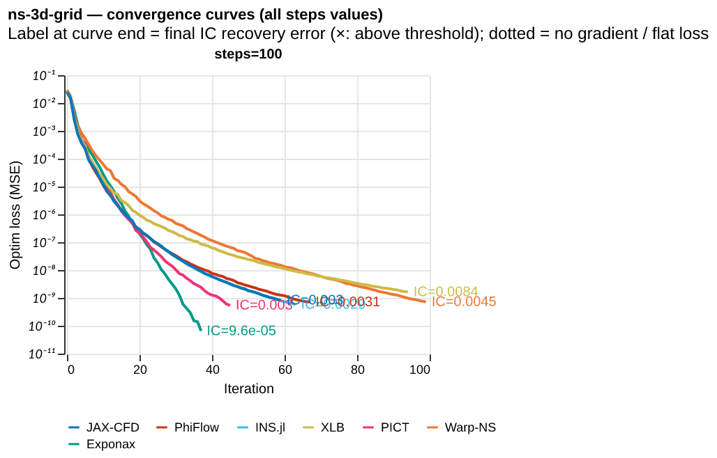
Final IC recovery error per solver from zero-initialised L-BFGS optimisation with divergence-free projection.